LArSoft
Software for Liquid Argon time projection chambers
PreV10 Geometry Package
Different detectors are represented in the Geometry Package of LArSoft. This information applies to versions before version 10 of LArSoft.
How a LArTPC works
Since neutrino interactions with matter are rare, physicists operate detectors with massive amounts of target material for runs lasting many years. Collisions between neutrinos and atoms in the target material produce particles which can be detected. Cosmic rays and other backgrounds also produce particles which must be distinguished from those produced by the neutrino interactions. The detectors record the tracks of charged particles traversing them. A conceptual view of the detection process in a single-phase Liquid Argon Time Projection Chamber (LArTPC) is available in the following 30-second animation: https://www.youtube.com/watch?v=R5G1_hW0ZUA. In contrast to the timescale shown in the animation, in a real detector the ionization drifts at a speed that is orders of magnitude slower than the velocity of the muon. As a result, the ionization left in the detector retains the shape of the deposited charge in space, thereby creating a 3D image of the energy deposition from all of the charged particles created in the interaction. This agglomeration then drifts (more or less) intact to the anode plane. The time at which the drifting electrons arrive at the anode can be measured, and if the production time is known, then the distance from the anode to the production point can be established.
LArTPCs are particle detectors that use electric fields, and possibly magnetic fields, in a large volume of liquid argon within a cryostat to obtain multiple two-dimensional images of particle trajectories. One goal of reconstruction software is to form a three-dimensional model of an interaction based on the two-dimensional information recorded by the detector. A time projection chamber (TPC) is constructed of an anode plane, a cathode plane and a field cage that shapes the electric field between them. Large detectors are modular and may have multiple cathode and anode planes. Within a detector, a series of anode plane assemblies may be installed next to each other to form one large anode plane. Anode plane assemblies are abbreviated APAs and cathode plane assemblies are abbreviated CPAs.
When a bias voltage is applied, an approximately uniform electric field is created in the volume between the anode and cathode planes. A charged particle traversing this volume leaves a trail of ionization in the ultra-pure liquid argon. The electrons drift toward the anode plane, inducing electric currents in planes of sensing wires or some other sensing structure located near or on the anode plane. The current-signal waveforms from all sensing elements are amplified and digitized by front-end electronics and transmitted through immersed cables to a data acquisition (DAQ) system outside the cryostat. Scintillation light created along the path of ionization is observed by photodetectors, and provides the absolute time of the event.
Experiments may have more than one kind of LArTPC:
- In a single-phase LArTPC, the anode is composed of wire planes or other sensing elements in the liquid argon volume. The electric field and drift direction of most single-phase TPCs is directed horizontally.
- In a dual-phase LArTPC, ionization charge is extracted from the liquid, then amplified and detected in gaseous argon above the liquid surface. In a dual-phase TPC, the drift direction must be vertical or close to it because the liquid-gas boundary is horizontal.
Due to the small drift velocity in liquid argon, the Lorentz angle for useful magnetic fields is very small and is usually neglected. Space-charge buildup can affect the local drift direction and make it differ from the average applied electric field however. The effect of space charge on the electron drift is parameterized as a distortion in the arrival times and locations of the drifting charge as a function of the production point.
To fully support any TPC, arbitrary electric field and drift directions must be supported.
How LArSoft geometry fits in
LArSoft is a simulation, reconstruction and analysis framework for LArTPCs. Currently, only anode planes with sense wires or strips are supported, though efforts based on LArSoft simulate pixel-based detectors are underway. Different detectors are represented in the LArSoft geometry.
The LArSoft geometry provides descriptions of the physical structures and materials in the detector. Some important specifiable parameters in the detector geometry include:
- the position of the detector relative to the beam
- the structure and material properties of the cathode planes
- where individual photon detectors are
- the placement of wires and the distance between them within a plane
- the distances between the wire planes
- the details of the material surrounding the cryostat
- the composition of the overburden
- transformations between coordinate systems attached to various elements and global coordinates
The geometry also provides a mapping between sensing elements such as wires or strips and DAQ channels.
Geometry model in LArSoft
The geometry description is hierarchically organized, with volume names and containership relations shown in Figure 1.
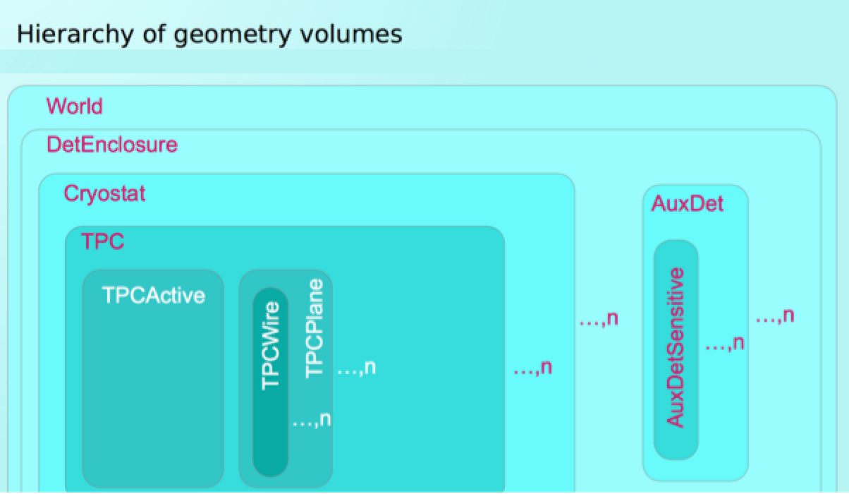
Figure 1: LArSoft’s geometry volume hierarchy diagram. Each instance can be repeated multiple times, indicated by the …n labels, though n can be different for each kind of volume.
A volume is the space contained within a set of closed surfaces. In the LArSoft Geometry, there is a hierarchy of volumes. Within each volume, there is a set of structures that are described, each of which may contain other volumes. Details about the lower-level volumes are found inside each element. Naming conventions are shown in Figure 1: volumes are named “vol” + name from Figure 1 + additional characters specifying which instance it is. Examples are given below.
- The World volume volWorld contains everything else including DetEnclosure and surrounding material. It contains all elements of the geometry that are to be accounted for in the simulation and should be sized adequately to account for any features of the detector surroundings that are important for the simulation. For example, if there is a mass of rock near the detector that could alter the cosmic ray flux, it should be simulated. One has a choice of parameterizing the cosmic-ray flux at a fixed surface instead of using GEANT, as GEANT may not be the most efficient or correct program for propagating muons through very long distances of rock. The volWorld has only one instance and contains volDetEnclosure.
- Detector Enclosure (volDetEnclosure) contains the cryostat and auxiliary detectors. It must be unique.
- Cryostat is a description of all the material that is the cryostat. In MicroBooNE, there is a description of a cylinder with end caps. In DUNE, cryostats are rectangular prisms. In LArSoft geometry, the cryostat is of arbitrary shape and size. The class that represents the cryostat needs to be able to describe any cryostat shape. It can contain many TPCs.
- Time Projection Chamber (volTPC) has a drift volume, a uniform electric field, and is read out by the wires within a single anode frame. The use of TPC in LArSoft comes from the time when every experiment had one TPC. With larger detectors, this may be better referred to as a ‘Drift volume’ since it may not have walls whereas a TPC does. Each TPC contains only one volTPCActive and many volTPCPlaneXXX volumes.
- volTPCActive defines the active volume of liquid argon in which drifting ionization and scintillation photons are simulated. Any liquid argon that is outside of the drift field would not be part of volTPCActive, but it still contributes to energy loss, showering, and all of GEANT’s physics processes; it just doesn’t contribute to the readout. Moreover, it is assumed that volTPCActive is simply a volume, i.e. a box, of liquid argon with no subvolumes inside. If we want the argon between the wire planes to be active, the GEANT4 region can be extended to handle this, but it requires changes to the current code. The thought is that this would only be required for single-phase because its the one that has an inter-plane region that could be sensitive.
- volTPCWire describes a wire segment in the detector. The word wire refers to a straight segment of a physical wire in one TPC. A wire that wraps around an APA frame consists of several of these segments.
- volTPCPlane describes a wire plane in the detector. It ends at the boundaries of the Anode Plane Assembly.
- volOpDetSensitive describes optical detectors’ sensitive elements.
- volAuxDet represents auxiliary detectors.
- volAuxDetSensitive is associated with the sensitive elements of the auxiliary detectors. These are typically used for cosmic-ray taggers or beam-related detectors.
Most of these elements are represented in LArSoft by a class for that type of element (geo::CryostatGeo, geo::TPCGeo, …). Each of the cryostats, TPCs, planes and wires has its own instance.
What you can do with the geometry
The geometry package contains classes related to the geometry representation. Classes represent planes, TPCs, cryostats. Geometry service and geometry services provider, Geometry-core, are in the geometry package as well as classes that perform sorting functions for experiments.

Wire base (in geo::PlaneGeo), geometry information for a single readout plane. Knowing a position in the detector, can know how it relates to the wire planes. So can figure out how far it is from the plane, what is the nearest wire along the nominal drift direction, etc.

Frame base (also in geo::PlaneGeo): Given how the point relates to the frame of the plane, can determine how the point relates to the wires on the plane.
Can get things like the drift distance from the plane pid.
geo::PlaneGeo const& plane = geom.Plane(pid);
double driftDistance = plane.DistanceFromPlane(p);
To get the nearest channel, one uses GeometryCore:
TVector3 p_inside = geom.Plane(pid).MovePointOverPlane(p);
raw::ChannelID_t channel = geom.NearestChannel(p_inside, pid);
because geo::PlaneGeo is not supposed to know about channels. Experiment-specific details are provided in a later section.
The geometry service provides access to information within LArSoft via methods that give answers to particular questions. Each function relies on the underlying geometry. Most geometry methods accept objects of type TVector3 for points and vectors.
Questions that can be answered:
- Which TPC contains the point
P?
To represent the point and find its TPC, the developer can use a vector object.
geo::TPCID tpcid = geom.FindTPCAtPosition(P);
If the pointof_interestdoesn’t reside in any of the TPCs, the returned id (tpcid) is ‘invalid’. This can be checked viatpcid.isValidorbool(tpcid). - What is the drift distance of point
Qfrom the wire planepid?
This information is extracted from the plane object.
geo::PlaneGeo const& plane = geom.Plane(pid);
double driftDistance = plane.DistanceFromPlane(Q);
The variabledriftDistancecontains the information on the drift distance. - Where is a cluster of ionized electrons at point
Cafter drifting by 10.5 centimeters?
Let theTPCobject translate it (note that it’s 10.5 cm closer to the anode):
geo::TPCGeo const& TPC = geom.TPC(tpcid);
TPC.DriftPoint(C, 10.5);
The content of the variableCis updated to contain the value of the translated point.
Plane objects can do the same:
geo::PlaneGeo const& plane = geom.Plane(pid);
plane.DriftPoint(C, 10.5);
Now, the content of the variablecheckingcontains the value of the translated point. - How to know if projection of point
where_is_thisfalls inside planepid?
This information is extracted from the plane object:
bool onPlane = geom.Plane(pid).isProjectionOnPlane(where_is_this); - How to find the point closest to point
var_pon planepid?
The plane can “move” a point (or projection) to the closest border when it’s out of it:
TVector3 p_inside = geom.Plane(pid).MovePointOverPlane(var_p);
The result is guaranteed to be inside the plane (pointvar_pis unchanged). - What is the wire coordinate of point
this_pointon planepid? This is looking for a real number expressing the position of the point projection on the wires. For example, if the project falls on wire number 5, we expect the result to be 5.0.
double wc1 = geom.Plane(pid).WireCoordinate(this_point);
double wc2 = geom.WireCoordinate(this_point, pid);
There are two methods here: the first queries the plane object (obtained withgeom.Plane(pid)), while the second goes directly to the geometry service provider. They are equivalent, but you may prefer the first one if you need to do more things with the plane object afterwards, or if you have that object available already (in which case you don’t need to discover it with thegeom.Plane(pid)query either).
Note: this is different from the legacyWireCoordinate(y, z)(inGeometryCoreandChannelMapAlg), which takes only two coordinates as arguments. The new method is universal and takes a complete 3D point.
If we wanted the same projection measured in centimetres (wc):
double wc1 = geom.Plane(pid).PlaneCoordinate(this_point);
and for a point on wire 5 on a 0.3 mm pitch plane, we would get 1.5 (centimeters). - How to find the wire closest to point
of_intereston planepid?
By putting together the recipes above:
geo::PlaneGeo const& plane = geom->Plane(pid);
geo::WireID wid = plane.NearestWireID(plane.MovePointOverPlane(of_interest));
(usingGeometryCore::NearestWireID()is equivalent here but slightly less efficient because the plane needs to be found twice).
To get the nearest channel, instead, one has to go viaGeometryCore: TVector3 p_inside = geom.Plane(pid).MovePointOverPlane(of_interest); raw::ChannelID_t channel = geom.NearestChannel(p_inside, pid);
becausegeo::PlaneGeois not supposed to know about channels. - I measured a hit on wire a of plane
band a hit on wirecon planedand they describe the same energy deposit. What should I find on planeewhich is another view of the same information?
Since you have three views, checking the other plane would help you determine if your information is consistent so you can be more confident that your assumption that they describe the same energy deposit is correct.
Answer: Not implemented, so far. - Where do wires
eandfintersect?
Nowhere. A projection plane must be defined, and a coordinate system on it to correctly express a “where”. The physical wires do not intersect. You want to know where they look like they intersect, but you need a projection plane for that. - I measured a hit on wire
aof planeband a hit on wirecon planesand they describe the same energy deposit. I also measured the drift distanced. Where was the energy deposited in space?
Answer: Not implemented. - Which are the coordinates of point
of_intereston planepid?
Assuming we are talking of the plane frame:
geo::PlaneGeo::WidthDepthProjection_t proj = geom.Plane(pid).PointWidthDepthProjection(of_interest);
double w_coord = proj.X(), d_coord = proj.Y();
LArSoft geometry evolution
LArSoft release 6.28 changed the geometry to support dual-phase TPCs, which caused several assumptions to be removed or to change:
- the drift direction is no longer assumed to be along x, but can be on any axis
- the projection of a point on a plane is no longer assumed to have coordinates (y,z)
- views no longer are assumed to measure a coordinate growing with z
- the outer plane cannot be assumed to have drift coordinate 0 (same as drift distance)
When updating code, understanding the assumptions at the time the code was written may help explain why certain options were chosen.
Note, that with ProtoDUNE Dual Phase, drift direction is necessarily upward (+y).
Detector description elements are present at many levels:
- source GDML file (needed by Geant4), optionally ROOT file too
- ROOT via TGeoManager, ROOT owns a complete translation of the source in terms of TGeoVolume objects
- LArSoft has a reduced translation that includes specific classes for wires, TPCs, and other relevant components
- Geant4 will own its own representation out of the source when run

The existing geometry model has two services when configuring:
geo::Geometry(service provider:geo::GeometryCore): people interactions- manages the ROOT geometry description and its GDML source
- provides access to LArSoft description of detector components
- facilitates iteration on detector components by type
- describes relations between components
- delegates to its “channel mapping” algorithm:
- mapping logical readout channels and wires
- view and signal type of planes
- “wire coordinate” of a point, nearest wire
geo::ExptGeoHelperInterface:experiment customization- implemented by each experiment (“standard” available)
- chooses the implementation of channel mapping (
geo::ChannelMapAlg) - chooses the procedures to sort geometry elements (
geo::GeoObjectSorter)
Most geometry functionality is now in geo::GeometryCore.
More than one wire might be in the same TPC readout channel when TPCs share APAs. For experiments, like MicroBooNE, whose TPCs don’t share APAs, each channel is assigned to a single wire. ProtoDUNE dual-phase has multiple TPCs but don’t share APAs. (Single-phase has multiple TPCs that do share APAs.) The code used to assume that each wire was on one TPC readout channel, but that assumption is no longer valid.
The abstraction of drift direction can be framed in a broader context. The drift direction is from the TPC active volume to the wire planes ⇒ owned by the TPC, defined by the geometry source. The coordinate measured by a wire plane (“wire coordinate”, wc) is orthogonal to the wires ⇒ owned by the plane, defined by the geometry sorting. Plane “width” and “depth” directions follow the plane frame sides ⇒ owned by the plane, defined by geometry source + convention. We still make some basic assumptions:
- y is “up” (where cosmic rays pour from)
- drift direction orthogonal to the planes
- perfectly spaced rigid wires
- shape of wire plane frame is rectangle
Writing and visualizing your own geometry
The Geometry Description Markup Language is an application-independent geometry description format based on XML. https://gdml.web.cern.ch/GDML/ There exist two toolkit bindings for GDML, the Geant4 binding and the ROOT binding, both integrated within the respective frameworks. Both bindings support reading and writing GDML files.
The GDML manual provides the structure and commands. (They’re called tags in GDML.) The Geant4 binding for GDML begins with three examples, which demonstrate the reading and writing out of different geometry configurations from/to GDML files. Instructions on how to visualize GDML files outside of LArSoft using Geant4 locally can be found in the Geant4 User Documentation. The main advantage of using one of the built-in examples of Geant4 to visualize a GDML file is a menu listing all components of the geometry described in the GDML file. This menu makes it easy for the user to display or hide specific parts of the geometry without knowing a priori which name was designated to them.
The ROOT binding for GDML is integrated within the ROOT framework. Information on importing or exporting GDML files can be found in the general ROOT manual. But the description of the GDML Schema is application-independent and therefore is relevant for both Geant4 and ROOT users.
For a simple example, set up a ROOT installation, taking special care of using the —enable-gdml option when compiling. You may want to example ROOT’s web catalog on how to load a gdml file using the TGeoManager class:
https://root.cern.ch/doc/master/classTGeoManager.html
The simplest way is:
{
gSystem->Load("libGeom");
gSystem->Load("libGdml");
TGeoManager::Import("myfile.gdml");
gGeoManager->FindVolumeFast("volWorld")->Draw("ogl");
}
This will display your geometry onscreen, supposing your World Volume is named volWorld. Note, the string ‘volWorld’ relates back to the description of Figure 1. The code can be searched to find strings that are used in the GDML files. For a given detector, experiments maintain their detector-geometry description in GDML files. The concepts behind GDML (such as the hierarchy of shapes, materials, and physical volumes) will be familiar to anyone who’s worked with other physics modeling packages, such as Geant4 or GeoModel. In LArSoft, the use of GDML is affected by the need to preserve geometry files associated with existing detectors and some limitations with ROOT.